Usage
plot_sr_ev(
  sro = NULL,
  fpage = 1,
  fcol = "id",
  xcol = "time",
  error_msgs = NULL,
  ylog = TRUE,
  ylab_str = "Amount",
  xlab_str = "Time",
  post_proc = "fig  = fig + ggplot2::theme_light()",
  evplot = c(1, 4),
  fncol = 4,
  fnrow = 2
)

plot_sr_ev(
  sro = NULL,
  fpage = 1,
  fcol = "id",
  xcol = "time",
  error_msgs = NULL,
  ylog = TRUE,
  ylab_str = "Amount",
  xlab_str = "Time",
  post_proc = "fig  = fig + ggplot2::theme_light()",
  evplot = c(1, 4),
  fncol = 4,
  fnrow = 2
)
Arguments
- sro
Output of 'simulate_rules()'.
- fpage
If facets are selected and multiple pages are generated then this indcates the page to return.
- fcol
Name of column to facet by or
NULLto disable faceting ("id").- xcol
Name of column to take x-data from (
"time").- error_msgs
Named list with error messages to overwrite (
NULL- ylog
Boolean to enable log10 scaling of the y-axis (
TRUE- ylab_str
Label for the y-axis (
"Output"- xlab_str
Label for the x-axis (
"Output"- post_proc
Character object with post processing post-processing code for the figure object named
figinternall ("fig = fig + theme_light()")- evplot
Evids to plot can be 1 or 4
- fncol
Number of columns in faceted output.
- fnrow
Number of rows in faceted output.
Value
List with the followin1g elements:
isgood: Return status of the function.
msgs: Error or warning messages if any issues were encountered.
npages: Total number of pages using the current configuration.
error_msgs: List of error messages used.
dsp: Intermediate dataset generated from
sroto plot in ggplot.fig: Figure generated.
Details
For a detailed examples see vignette("clinical_trial_simulation", package = "ruminate").
For a detailed examples see vignette("clinical_trial_simulation", package = "ruminate").
Examples
# \donttest{
library(formods)
library(ggplot2)

# For more information see the Clinical Trial Simulation vignette:
# https://ruminate.ubiquity.tools/articles/clinical_trial_simulation.html

# None of this will work if rxode2 isn't installed:
if(is_installed("rxode2")){
library(rxode2)
set.seed(8675309)
rxSetSeed(8675309)

my_model = function ()
{
    description <- "One compartment PK model with linear clearance using differential equations"
    ini({
        lka <- 0.45
        label("Absorption rate (Ka)")
        lcl <- 1
        label("Clearance (CL)")
        lvc <- 3.45
        label("Central volume of distribution (V)")
        propSd <- c(0, 0.5)
        label("Proportional residual error (fraction)")
        etalcl ~ 0.1
    })
    model({
        ka <- exp(lka)
        cl <- exp(lcl + etalcl)
        vc <- exp(lvc)
        kel <- cl/vc
        d/dt(depot) <- -ka * depot
        d/dt(central) <- ka * depot - kel * central
        Cc <- central/vc
        Cc ~ prop(propSd)
    })
}

# This creates an rxode2 object
object  = rxode(my_model)

# If you want details about the parameters, states, etc
# in the model you can use this:
rxdetails = fetch_rxinfo(object)

rxdetails$elements

# Next we will create subjects. To do that we need to
# specify information about covariates:
nsub = 2
covs = list(
  WT         = list(type     = "continuous",
                    sampling = "log-normal",
                    values   = c(70, .15))
)

subs = mk_subjects(object = object,
                   nsub   = nsub,
                   covs   = covs)

head(subs$subjects)

rules = list(
  dose = list(
    condition = "TRUE",
    action    = list(
      type  = "dose",
      state     = "central",
      values    = "c(1)",
      times     = "c(0)",
      durations = "c(0)")
    )
)

# We evaulate the rules for dosing at time 0
eval_times =  0

# Stop 2 months after the last dose
output_times = seq(0, 56, 1)

# This runs the rule-based simulations
simres =
  simulate_rules(
    object        = object,
    subjects      = subs[["subjects"]],
    eval_times    = eval_times,
    output_times  = output_times,
    rules         = rules)

# First subject data:
sub_1 = simres$simall[simres$simall$id == 1, ]

# First subjects events
evall = as.data.frame(simres$evall)
ev_sub_1 = evall[evall$id ==1, ]

# All of the simulation data
simall = simres$simall
simall$id = as.factor(simall$id)

# Timecourse
psim =
  plot_sr_tc(
    sro    = simres,
    dvcols = "Cc")
psim$fig

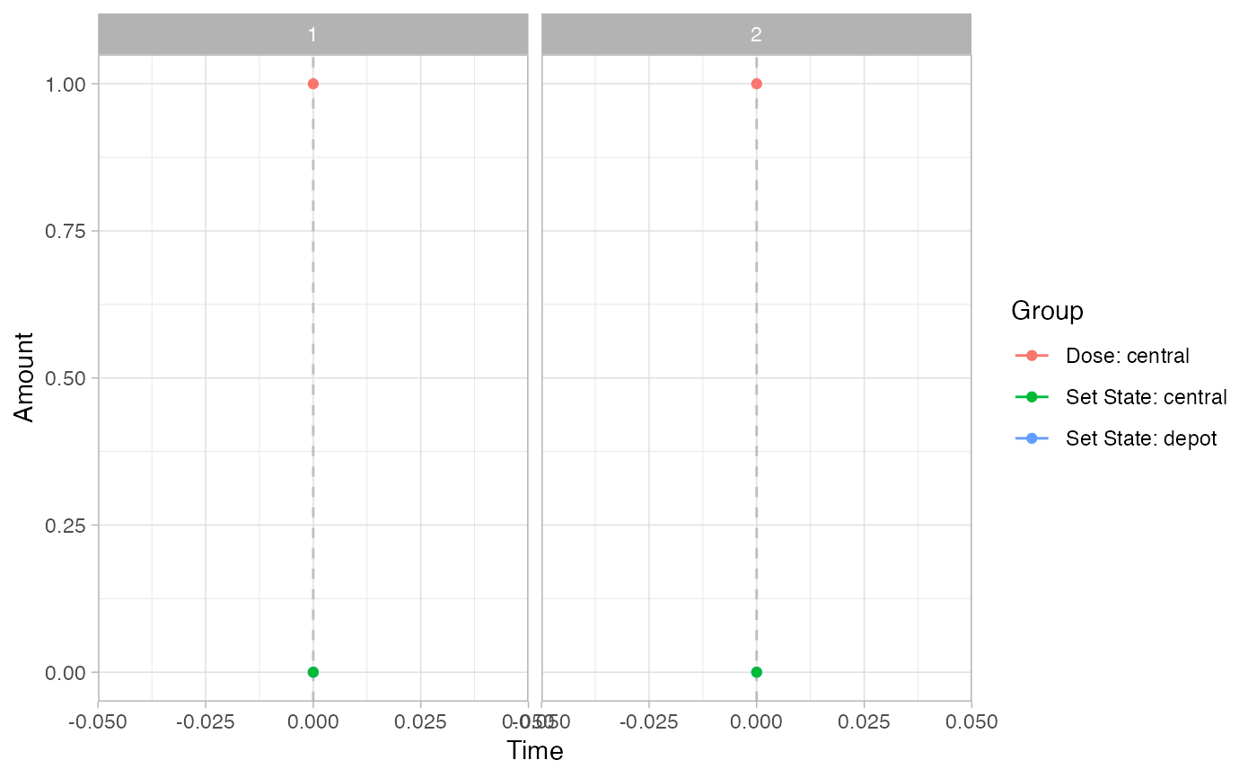
# Events
pev =
  plot_sr_ev(
    sro    = simres,
    ylog   = FALSE)
pev$fig

}
#>
#>
#> ℹ parameter labels from comments are typically ignored in non-interactive mode
#> ℹ Need to run with the source intact to parse comments
#>
#>
#>
#>
#> Warning: multi-subject simulation without without 'omega'
#>
#>
#> Warning: multi-subject simulation without without 'omega'
#> `geom_line()`: Each group consists of only one observation.
#> ℹ Do you need to adjust the group aesthetic?
#> `geom_line()`: Each group consists of only one observation.
#> ℹ Do you need to adjust the group aesthetic?

# }
# \donttest{
library(formods)
library(ggplot2)

# For more information see the Clinical Trial Simulation vignette:
# https://ruminate.ubiquity.tools/articles/clinical_trial_simulation.html

# None of this will work if rxode2 isn't installed:
if(is_installed("rxode2")){
library(rxode2)
set.seed(8675309)
rxSetSeed(8675309)

my_model = function ()
{
    description <- "One compartment PK model with linear clearance using differential equations"
    ini({
        lka <- 0.45
        label("Absorption rate (Ka)")
        lcl <- 1
        label("Clearance (CL)")
        lvc <- 3.45
        label("Central volume of distribution (V)")
        propSd <- c(0, 0.5)
        label("Proportional residual error (fraction)")
        etalcl ~ 0.1
    })
    model({
        ka <- exp(lka)
        cl <- exp(lcl + etalcl)
        vc <- exp(lvc)
        kel <- cl/vc
        d/dt(depot) <- -ka * depot
        d/dt(central) <- ka * depot - kel * central
        Cc <- central/vc
        Cc ~ prop(propSd)
    })
}

# This creates an rxode2 object
object  = rxode(my_model)

# If you want details about the parameters, states, etc
# in the model you can use this:
rxdetails = fetch_rxinfo(object)

rxdetails$elements

# Next we will create subjects. To do that we need to
# specify information about covariates:
nsub = 2
covs = list(
  WT         = list(type     = "continuous",
                    sampling = "log-normal",
                    values   = c(70, .15))
)

subs = mk_subjects(object = object,
                   nsub   = nsub,
                   covs   = covs)

head(subs$subjects)

rules = list(
  dose = list(
    condition = "TRUE",
    action    = list(
      type  = "dose",
      state     = "central",
      values    = "c(1)",
      times     = "c(0)",
      durations = "c(0)")
    )
)

# We evaulate the rules for dosing at time 0
eval_times =  0

# Stop 2 months after the last dose
output_times = seq(0, 56, 1)

# This runs the rule-based simulations
simres =
  simulate_rules(
    object        = object,
    subjects      = subs[["subjects"]],
    eval_times    = eval_times,
    output_times  = output_times,
    rules         = rules)

# First subject data:
sub_1 = simres$simall[simres$simall$id == 1, ]

# First subjects events
evall = as.data.frame(simres$evall)
ev_sub_1 = evall[evall$id ==1, ]

# All of the simulation data
simall = simres$simall
simall$id = as.factor(simall$id)

# Timecourse
psim =
  plot_sr_tc(
    sro    = simres,
    dvcols = "Cc")
psim$fig

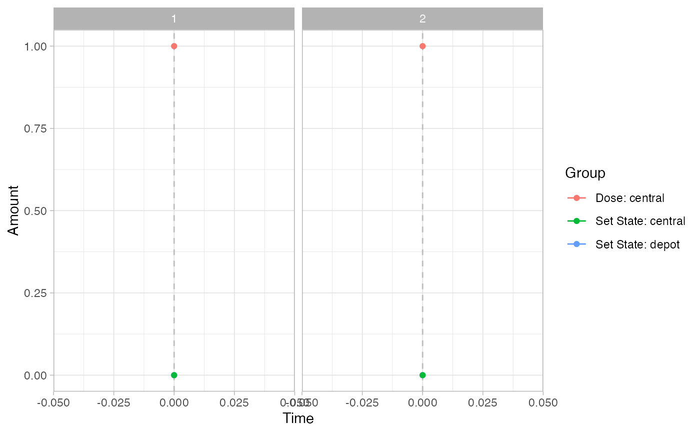
# Events
pev =
  plot_sr_ev(
    sro    = simres,
    ylog   = FALSE)
pev$fig

}
#>
#>
#> ℹ parameter labels from comments are typically ignored in non-interactive mode
#> ℹ Need to run with the source intact to parse comments
#>
#>
#>
#>
#> Warning: multi-subject simulation without without 'omega'
#> Evaluation times ■■■■■■■■■■■■■■■■                  50% | ETA:  3s
#>
#>
#> Warning: multi-subject simulation without without 'omega'
#> Evaluation times ■■■■■■■■■■■■■■■■■■■■■■■■■■■■■■■  100% | ETA:  0s
#> `geom_line()`: Each group consists of only one observation.
#> ℹ Do you need to adjust the group aesthetic?
#> `geom_line()`: Each group consists of only one observation.
#> ℹ Do you need to adjust the group aesthetic?

# }
# }
